Or why data analytics depends on data preparation.
I wanted to find the “Reach” of some Facebook groups. In my mind, it should have been a simple SUM calculation. It should have been an easy formula using Excel’s Sum Function. We can add all the values of “# of Members” up to get a total. So I open my staff’s FB groups list in XLSX format. And boy was I wrong!
Column A contains the FBgroup name (anonymized) and Column B contains the number of members for each group. This is shown below:
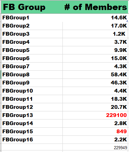
Your eyes immediately spy the fact that the numbers are in different formats. Some numbers are expressed in Ks (1000s). Other numbers are expressed as normal numerals. I highlighted these in red.
Apparently, Excel can’t sum up the values in Column B. Excel doesn’t know that K stands for 1000s. So the sum of the # of members (Reach) can’t be computed correctly. We would get an incorrect value of 229,949 members if we did a sum without processing the values in this column B.
This formula converts the “K” into 1000s. This means that 14.6K will become 14,600. We use the Find and LEFT function for this formula.
=IF(FIND(“K”,B2)>0,LEFT(B2,FIND(“K”,B2,1)-1)*1000,B2)
This formula searches for the letter “K” in the value of Column B. If K exist, then the result of Find(“K”,B2) will be greater than 0. When true, return the original value of B2 without the K (14.6) and then multiply it by 1000 to get 14,600.
However, if the K is not in the value of column B, then just return the column B value. For example, FBgroup13 has a value of 229100 (no K). So its value should hold 229100. And voila! We are now getting somewhere!

We are not yet done. While the ‘translated’ values of B2 are correctly listed in the column D (Column1), you see that for values in column B without “K”, the formula results in an error #Value! for the translated value column. I have highlighted these in red too.
Look at FBGroup13 should be 229,100 and the value for FBGroup15 should be 849. But both get #VALUE! instead. We solve this by creating a new column E (column2). Here we test for the Error condition.
=IFERROR(d2, b2)
If we get #Value! (or any error), just get the value from B2, otherwise, use the existing value of D2.

Now that we have converted the values into correct numbers, we can easily sum the total number of members for all FB groups. The correct number is 448,749.